> Simulation for decision analysis
```{r include = FALSE}
library(radiant.data)
```
Start by selecting the types of variables to use in the simulation from the `Select types` dropdown in the _Simulate_ tab. Available types include Binomial, Constant, Discrete, Log normal, Normal, Uniform, Data, Grid search, and Sequence.
### Binomial
Add random variables with a binomial distribution using the `Binomial variables` inputs. Start by specifying a `Name` (`crash`), the number of trials (n) (e.g., 20) and the probability (p) of a `success` (.01). Then press the icon. Alternatively, enter (or remove) input directly in the text input area (e.g., crash 20 .01).
### Constant
List the constants to include in the analysis in the `Constant variables` input. You can either enter names and values directly into the text area (e.g., `cost 3`) or enter a name (`cost`) and a value (5) in the `Name` and `Value` input respectively and then press the icon. Press the icon to remove an entry. Note that only variables listed in the (larger) text-input boxes will be included in the simulation.
### Discrete
Define random variables with a discrete distribution using the `Discrete variables` inputs. Start by specifying a `Name` (`price`), the values (6 8), and their associated probabilities (.3 .7). Then press the icon. Alternatively, enter (or remove) input directly in the text input area (e.g., price 6 8 .3 .7). Note that the probabilities must sum to 1. If not, a message will be displayed and the simulation cannot be run.
### Log Normal
To include log normally distributed random variables in the analysis select `Log Normal` from the `Select types` dropdown and use `Log-normal variables` inputs. See the section `Normal` below for additional information.
### Normal
To include normally distributed random variables in the analysis select `Normal` from the `Select types` dropdown and use `Normal variables` inputs. For example, enter a `Name` (`demand`), the `Mean` (1000) and the standard deviation (`St.dev.`, 100). Then press the icon. Alternatively, enter (or remove) input directly in the text input area (e.g., `demand 1000 100`).
### Poisson
The Poisson distribution is useful to simulate the number of times and event occurs in a particular time span, such as the number of patients arriving in an emergency room between 10 and 11pm. To include Poisson distributed random variables in the analysis select `Poisson` from the `Select types` dropdown and use `Poisson variables` inputs. For example, enter a `Name` (`patients`) and a value for the number of occurrences `Lambda` the event of interest (20). Then press the icon. Alternatively, enter (or remove) input directly in the text input area (e.g., `patients 20`).
### Uniform
To include uniformly distributed random variables in the analysis select `Uniform` from the `Select types` dropdown. Provide parameters in the `Uniform variables` inputs. For example, enter a `Name` (`cost`), the `Min` (10) and the `Max` (15) value. Then press the icon. Alternatively, enter (or remove) input directly in the text input area (e.g., `cost 10 15`).
### Data
To include variables from a separate data-set in the calculations specified in the `Simulation formulas` input box, choose a data-set from the `Input data for calculations` dropdown. This can be very useful in combination with the `Grid search` feature for portfolio optimization. However, when used in conjunction with other inputs care must be taken to ensure the number of values returned by different calculations is the same. Otherwise you will see an error like:
`Error: arguments imply differing number of rows: 999, 3000`
### Grid search
To include a sequence of values select `Grid search` from the `Select types` dropdown. Provide the minimum and maximum values as well as the step-size in the `Grid search` inputs. For example, enter a `Name` (`price`), the `Min` (4), `Max` (10), and `Step` (0.01) value. If multiple variables are specified in `Grid search` all possible value combinations will be created and evaluated in the simulation. For example, suppose a first variable is defined as `x 1 3 1` and a second as `y 4 5 1` in the `Grid search` text input then the following data is generated:
```{r results = 'asis', echo = FALSE}
x <- c(1, 2, 3)
y <- c(4, 5)
tab_large <- "class='table table-condensed table-hover' style='width:40%;'"
expand.grid(x, y) %>%
set_names(c("x", "y")) %>%
knitr::kable(align = "l", format = "html", escape = FALSE, table.attr = tab_large)
```
Note that if `Grid search` has been selected the number of values generated will override the number of simulations or repetitions specified in `# sims` or `# reps`. If this is not what you want use `Sequence`. Then press the icon. Alternatively, enter (or remove) input directly in the text input area (e.g., `price 4 10 0.01`).
### Sequence
To include a sequence of values select `Sequence` from the `Select types` dropdown. Provide the minimum and maximum values in the `Sequence variables` inputs. For example, enter a `Name` (`trend`), the `Min` (1) and the `Max` (1000) value. Note that the number of 'steps' is determined by the number of simulations. Then press the icon. Alternatively, enter (or remove) input directly in the text input area (e.g., `trend 1 1000`).
### Formulas
To perform a calculation using the generated variables, create a formula in the `Simulation formulas` input box in the main panel (e.g., `profit = demand * (price - cost)`). Formulas are used to add (calculated) variables to the simulation or to update existing variables. You must specify the name of the new variable to the left of a `=` sign. Variable names can contain letters, numbers, and `_` but no other characters or spaces. You can enter multiple formulas. If, for example, you would also like to calculate the margin in each simulation press `return` after the first formula and type `margin = price - cost`.
Many of the same functions used with `Create` in the _Data > Transform_ tab and in `Filter data` in _Data > View_ can also be included in formulas. You can use `>` and `<` signs and combine them. For example `x > 3 & y == 2` would evaluate to `TRUE` when the variable `x` has values larger than 3 **AND** `y` has values equal to 2. Recall that in R, and most other programming languages, `=` is used to _assign_ a value and `==` to evaluate if the value of a variable is exactly equal to some other value. In contrast `!=` is used to determine if a variable is _unequal_ to some value. You can also use expressions that have an **OR** condition. For example, to determine when `Salary` is smaller than \$100,000 **OR** larger than \$20,000 use `Salary > 20000 | Salary < 100000`. `|` is the symbol for **OR** and `&` is the symbol for **AND** (see also the help file for _Data > View_).
A few additional examples of formulas are shown below:
- Create a new variable z that is the difference between variables x and y
```r
z = x - y
```
- Create a new `logical` variable z that takes on the value TRUE when x > y and FALSE otherwise
```r
z = x > y
```
- Create a new `logical` z that takes on the value TRUE when x is equal to y and FALSE otherwise
```r
z = x == y
```
- The command above is equivalent to the one below using `ifelse`. Note the similarity to `if` statements in Excel
```r
z = ifelse(x < y, TRUE, FALSE)
```
- `ifelse` statements can be used to create more complex (numeric) variables as well. In the example below, z will take on the value 0 if x is smaller than 60. If x is larger than 100, z is set equal to 1. Finally, when x is 60, 100, or between 60 and 100, z is set to 2. **Note:** make sure to include the appropriate number of opening `(` and closing `)` brackets!
```r
z = ifelse(x < 60, 0, ifelse(x > 100, 1, 2))
```
- To create a new variable z that is a transformation of variable x but with mean equal to zero:
```r
z = x - mean(x)
```
- To create a new variable z that shows the absolute values of x:
```r
z = abs(x)
```
- To find the value for `price` that maximizes `profit` use the `find_max` command. In this example `price` could be a random or `Sequence variable`. There is also a `find_min` command.
```r
optimal_price = find_max(profit, price)
```
- To determine the minimum (maximum) value for each pair of values across multiple variables (e.g., x and y) use the functions `pmin` and `pmax`. In the example below, z will take on the value of x when x is larger than y and take on the value of y otherwise.
```r
z = pmax(x, y)
```
See the table below for an example:
```{r results = 'asis', echo = FALSE}
x <- c(1, 2, 3, 4, 5)
y <- c(0, 3, 8, 2, 10)
tab_large <- "class='table table-condensed table-hover' style='width:40%;'"
data.frame(
x = x,
y = y,
`pmax(x,y)` = pmax(x, y),
check.names = FALSE
) %>%
knitr::kable(align = "l", format = "html", escape = FALSE, table.attr = tab_large)
```
- Similar to `pmin` and `pmax` a number of functions are available to calculate summary statics across multiple variables. For example, `psum` calculates the sum of elements across different vectors. See https://radiant-rstats.github.io/radiant.data/reference/pfun.html for more information.
```r
z = psum(x, y)
```
See the table below for an example:
```{r results = 'asis', echo = FALSE}
x <- c(1, 2, 3, 4, 5)
y <- c(0, 3, 8, 2, 10)
tab_large <- "class='table table-condensed table-hover' style='width:40%;'"
data.frame(
x = x,
y = y,
`psum(x,y)` = psum(x, y),
check.names = FALSE
) %>%
knitr::kable(align = "l", format = "html", escape = FALSE, table.attr = tab_large)
```
Other commonly used functions are `ln` for the natural logarithm (e.g., `ln(x)`), `sqrt` for the square-root of x (e.g., `sqrt(x)`) and `square` to calculate square of a variable (e.g., `square(x)`).
To return a single value from a calculation use functions such as `min`, `max`, `mean`, `sd`, etc.
- A special function useful for portfolio optimization is `sdw`. It takes weights and variables as inputs and returns the standard deviation of the weighted sum of the variables. For example, to calculated the standard deviation for a portfolio of three stocks (e.g., Boeing, GM, and Exxon) you could use the equation below in the `Simulation formulas` input. `f` and `g` could be values (e.g., 0.2 and 0.8) or vectors of different weights specified in a `Grid search` input (see above). `Boeing`, `GM`, and `Exxon` are names of variables in a data-set included in the simulation using a `Data` input (see above).
```r
Pstdev = sdw(f, g, 1-f-g, Boeing, GM, Exxon)
```
For an example of how the simulate tool could be used for portfolio optimization see the state-file available for download here
### Functions
It is possible that the standard functions available in R are not sufficiently flexible to conduct the simulation you have in mind. If this is the case, click on the `Add functions` check box on the bottom left of your screen and can create your own custom function in the `Simulation functions` input box in the main panel. To learn about writing R-functions see https://www.statmethods.net/management/userfunctions.html for a good place to start.
For an example of how to use custom R-functions in a gambling simulation, see the state-file available for download here. The report generated through _Report > Rmd_ provides additional information about the simulation setup and the use of functions.
### Running the simulation
The value shown in the `# sims` input determines the number of simulation _draws_. To redo a simulation with the same randomly generated values, specify a number in the `Set random seed` input (e.g., 1234).
To save the simulated data for further analysis, specify a name in the `Simulated data` input box. You can then investigate the simulated data by choosing the data with the specified name from the `Datasets` dropdown in any of the _Data_ tabs (e.g., _Data > View_, _Data > Visualize_, or _Data > Explore_).
When all required inputs have been specified press the `Simulate` button to run the simulation.
In the screen shot below `var_cost` and `fixed_cost` are specified as constants. `E` is normally distributed with a mean of 0 and a standard deviation of 100. `price` is a discrete random variable that is set to \$6 (30% probability) or $8 (70% probability). There are three formulas in the `Simulation formulas` text-input. The first establishes the dependence of `demand` on the simulated variable `price`. The second formula specifies the profit function. The final formula is used to determine the number (and proportion) of cases where profit is below 100. The result is assigned to a new variable `profit_small`.
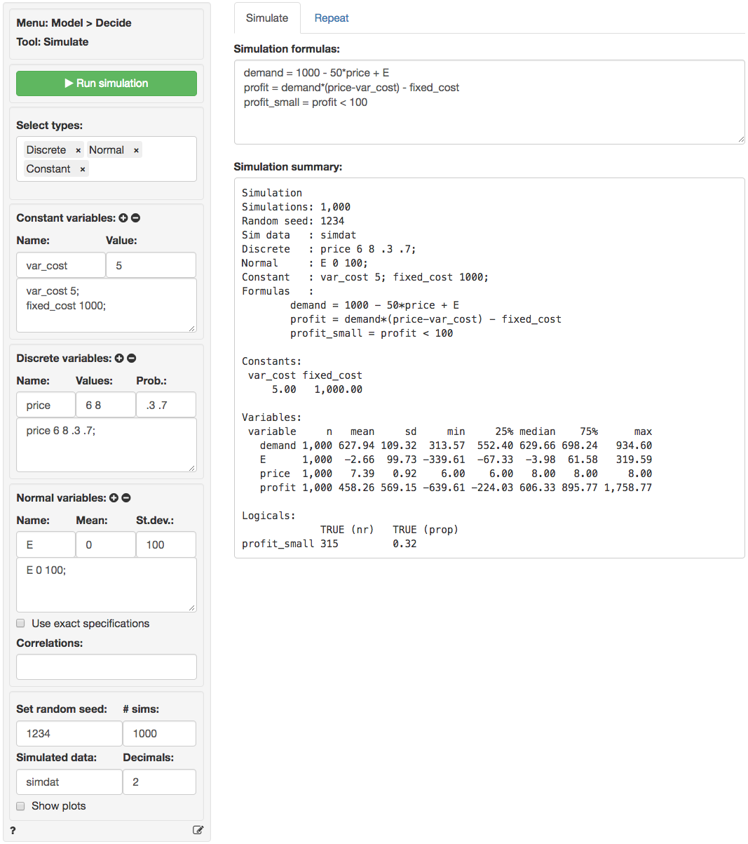
In the output under `Simulation summary` we first see details on the specification of the simulation (e.g., the number of simulations). The section `Constants` lists the value of variables that do not vary across simulations. The sections `Random variables` and `Logicals` list the outcomes of the simulation. We see that average `demand` in the simulation is 627.94 with a standard deviation of 109.32. Other characteristics of the simulated data are also provided (e.g., the maximum profit is 1758.77). Finally, we see that the probability of `profits` below 100 is equal 0.32 (i.e., profits were below \$100 in 315 out of the 1,000 simulations).
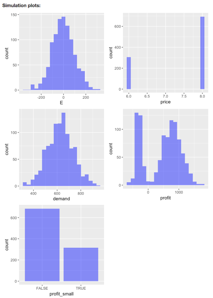
To view histograms of the random variables as well as the variables created using `Simulation formulas` ensure `Show plots` is checked.
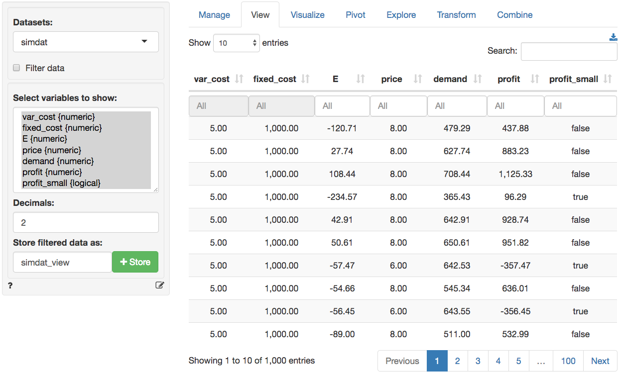
Because we specified a name in the `Simulated data` box the data are available as `simdat` within Radiant (see screen shots below). To use the data in Excel click the download icon on the top-right of the screen in the _Data > View_ tab or go to the _Data > Manage_ tab and save the data to a csv file (or use the clipboard feature). For more information see the help file for the _Data > Manage_ tab.
## Repeating the simulation
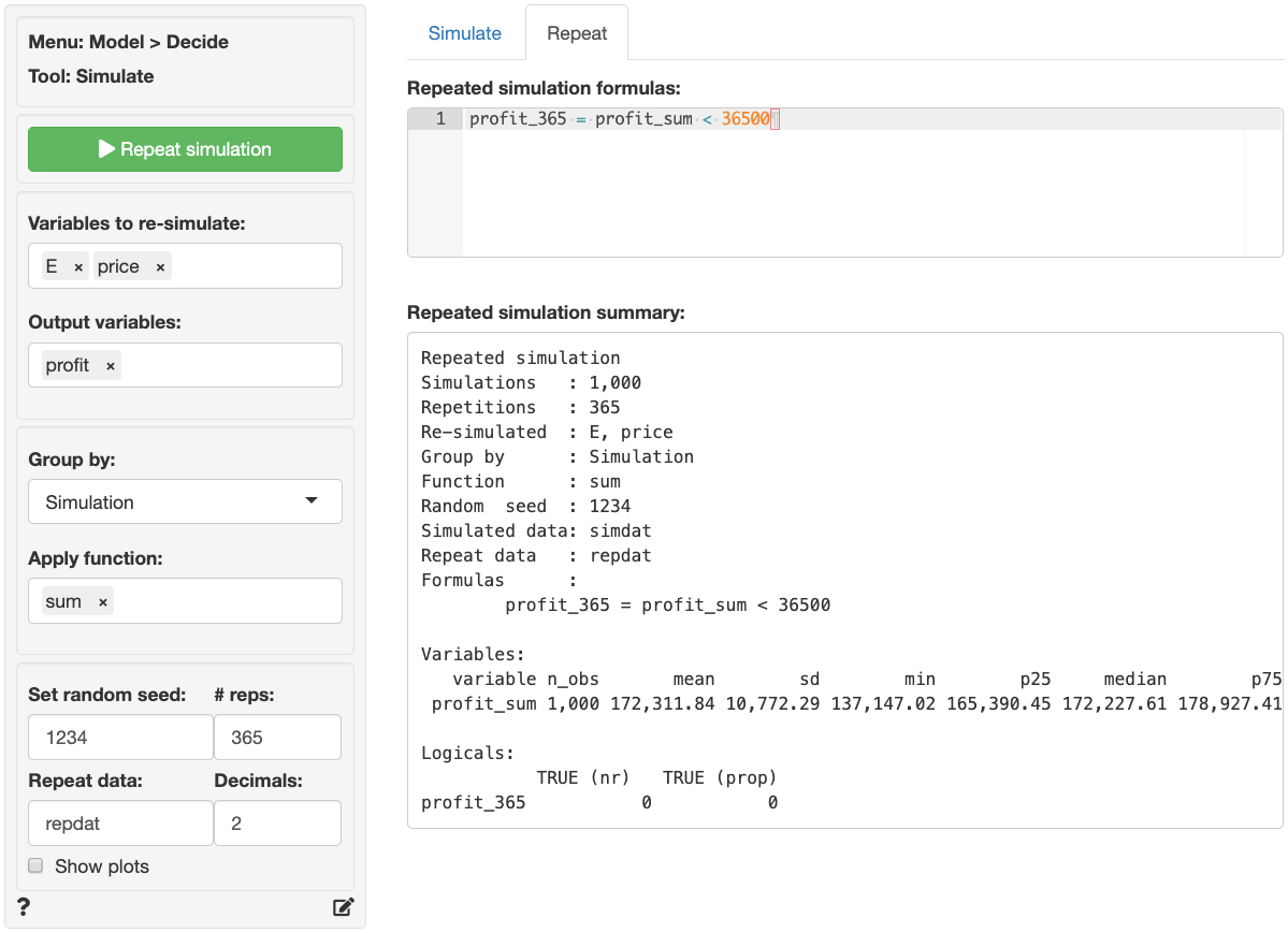
Suppose the simulation discussed above was used to get a better understanding of daily profits. To develop insights into annual profits we could re-run the simulation 365 times. However, this can be done more conveniently by using the functionality available in the _Repeat_ tab. First, select the `Variables to re-simulate`, here `E` and `price`. Then select the variable(s) of interest in the `Output variables` box (e.g., `profit`). Set `# reps` to 365.
Next, we need to determine how to summarize the data. If we select `Simulation` in `Group by` the data will be summarized for each draw in the simulation **across** 365 repeated simulations resulting in 1,000 values. If we select `Repeat` in `Group by` the data will be summarized for each repetition **across** 1,000 simulations resulting in 365 values. If you imagine the full set of repeated simulated data as a table with 1,000 rows and 365 columns, grouping by `Simulation` will create a summary statistic for each row and grouping by `Repeat` will create a summary statistic for each column. In this example we want to determine the `sum` of simulated daily profits across 365 repetitions so we select `Simulation` in the `Group by` box and `sum` in the `Apply function` box.
To determine, the probability that annual profits are below \$36,500 we enter the formula below into the `Repeated simulation formula` text input.
```r
profit_365 = profit_sum < 36500
```
Note that `profit_sum` is the `sum` of repeated simulations of the `profit` variable defined in the _Simulate_ tab. When you are done with the input values click the `Repeat` button. Because we specified a name for `Repeat data` a new data set will be created. `repdat` will contain the summarized data grouped per simulation (i.e., 1,000 rows). To store all 365 x 1,000 simulations/repetitions select `none` from the `Apply function` dropdown.
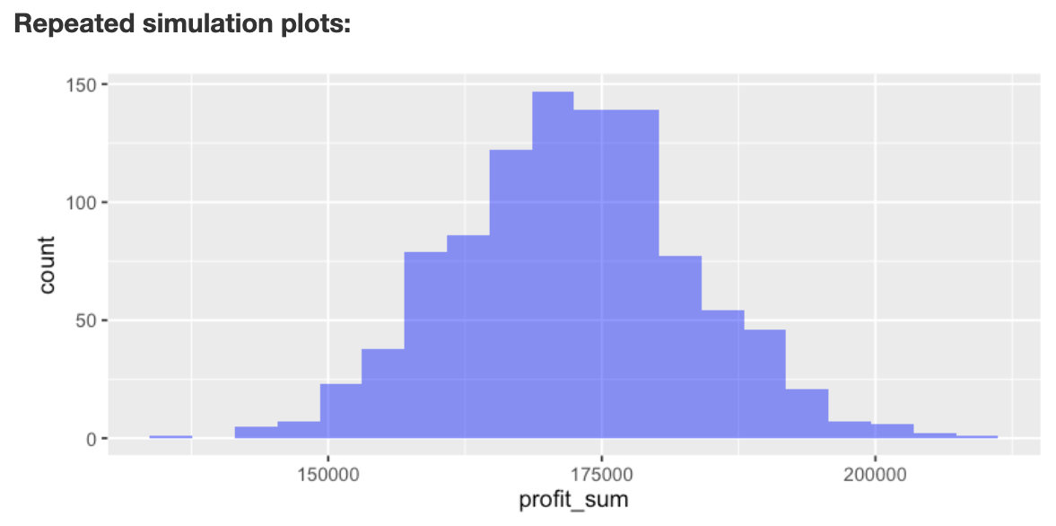
Descriptive statistics for the repeated simulation are shown in the main panel under `Repeated simulation summary`. We see that the annual expected profit (i.e., the mean of `profit_sum`) for the company is 172,311.84 with a standard deviation of 10,772.29. Although we found above that daily profits can be below \$100, the chance that profits are below $365 \times 100$ for the entire year are slim to none (i.e., the proportion of repeated simulations with annual profits below \$36,500 is equal to 0).
If `Show plots` is checked a histogram of annual profits (`profit_sum`) is shown under `Repeated simulation plots`. There is no plot for `profit_365` because it has only one value (i.e., FALSE).
The state-file for the example in the screenshots above is available for download here
For a simple example of how the simulate tool could be used to find the price that maximizes profits see the state-file available for download here
### Using Grid Search in the Repeat tab
Note that the _Repeat_ tab also has the option to use a `Grid search` input to repeat a simulation by replacing one or more `Constants` specified in the `Simulation` tab in an iterative fashion. This input option is shown only when `Group by` is set to `Repeat`. Provide the minimum and maximum values as well as the step-size in the `Grid search` inputs. For example, enter a `Name` (`price`), the `Min` (4), `Max` (10), and `Step` (0.01) value. If multiple variables are specified in `Grid search` all possible value combinations will be created and evaluated in the simulation. Note that if `Grid search` has been selected the number of values generated will override the number of repetitions specified in `# reps`. Then press the icon. Alternatively, enter (or remove) input directly in the text area (e.g., `price 4 10 0.01`).
### Report > Rmd
Add code to _Report > Rmd_ to (re)create the analysis by clicking the icon on the bottom left of your screen or by pressing `ALT-enter` on your keyboard.
If a plot was created it can be customized using `ggplot2` commands or with `patchwork`. See example below and _Data > Visualize_ for details.
```{r echo=TRUE, eval=FALSE}
plot(result, custom = TRUE) %>%
wrap_plots(plot_list, ncol = 2) + plot_annotation(title = "Simulation plots")
```
### R-functions
For an overview of related R-functions used by Radiant to construct and evaluate (repeated) simulation models see _Model > Simulate_.
Key functions from the `stats` package used in the `simulater` tool are `rbinom`, `rlnorm`, `rnorm`, `rpios`, and `runif`
### Video Tutorials
Copy-and-paste the full command below into the RStudio console (i.e., the bottom-left window) and press return to gain access to all materials used in the simulation module of the Radiant Tutorial Series:
usethis::use_course("https://www.dropbox.com/sh/72kpk88ty4p1uh5/AABWcfhrycLzCuCvI6FRu0zia?dl=1")
Setting Up a Simulation in Radiant (#1)
* This video demonstrates how to use Radiant to set up a simulation
* Topics List:
- Brief introduction to the Poisson distribution
- Specifying a simulation
- Interpretation of the simulation summary
Setting Up a Repeated Simulation in Radiant (#2)
* This video shows how to use Radiant to set up a repeated simulation
* Topics List:
- Specifying a repeated simulation
- Interpretation of the repeated simulation summary
Using simulation to solve probability questions (#3)
* This video demonstrates how to use simulation to solve probability questions in Radiant
* Topics List:
- Review of setting up a (repeated) simulation
- Interpretation of the simulation summary
- Intuition of how repeated simulations work
Simulation Formula Tips (#4)
* This video discusses some helpful functions that are commonly used in simulation formulas
* Topics List:
- Use `ifelse` to specify a simulation formula
- Use `pmax` to specify a simulation formula
Using Grid Search in Simulation (#5)
* This video demonstrates how to use grid search in simulation
* Topics List:
- Find an optimal value by sorting simulated data or create a plot
- Find an optimal value by using the `find_max` function