> A goodness-of-fit test is used to determine if data from a sample are consistent with a hypothesized distribution

### Example

The data are from a sample of 580 newspaper readers that indicated (1) which newspaper they read most frequently (USA today or Wall Street Journal) and (2) their level of income (Low income vs. High income). The data has three variables: A respondent identifier (id), respondent income (High or Low), and the primary newspaper the respondent reads (USA today or Wall Street Journal).

The data were collected to examine if there is a relationship between income level and choice of newspaper. To ensure the results are generalizable it is important that sample is representative of the population of interest. It is known that in this population the relative share of US today readers is higher than the share of Wall Street Journal readers. The shares should be 55% and 45% respectively. We can use a goodness-of-fit test to examine the following null and alternative hypotheses:

* H0: Readership shares for USA today and Wall Street Journal are 55% and 45% respectively
* Ha: Readership shares for USA today and Wall Street Journal are not equal to the stated values

If we cannot reject the null hypothesis based on the available sample there is a "good fit" between the observed data and the assumed population shares or probabilities. In Radiant (_Basics > Tables > Goodness of fit_) choose Newspaper as the categorical variable. If we leave the `Probabilities` input field empty (or enter 1/2) we would be testing if the shares are equal. However, to test H0 and Ha we need to enter `0.45 and 0.55` and then press `Enter`. First, compare the observed and expected frequencies. The expected frequencies are calculated assuming H0 is true (i.e., no deviation from the stated shares) as total $\times$ $p$, where $p$ is the share (or probability) assumed for a cell.

<p align="center"><img src="https://radiant-rstats.github.io/docs/basics/figures_basics//goodness_summary.png"></p>

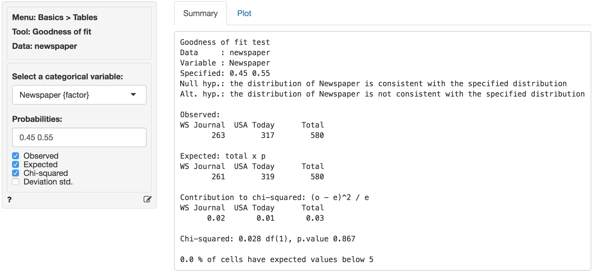
The (Pearson) chi-squared test evaluates if we can reject the null-hypothesis that the observed and expected values are the same. It does so by comparing the observed frequencies (i.e., what we actually see in the data) to the expected frequencies (i.e., what we would expect to see if the distribution of shares is as we assumed). If there are big differences between the table of expected and observed frequencies the chi-square value will be _large_. The chi-square value for each cell is calculated as `(o - e)^2 / e`, where `o` is the observed frequency in a cell and `e` is the expected frequency in that cell if the null hypothesis holds. These values can be shown by clicking the `Chi-squared` check box. The overall chi-square value is obtained by summing across all cells, i.e., it is the sum of the values shown in the _Contribution to chi-square_ table.

In order to determine if the chi-square statistic can be considered _large_ we first determine the degrees of freedom (df = # cells - 1). In a table with two cells we have df = (2-1) = 1. The output in the _Summary_ tab shows the value of the chi-square statistic, the df, and the p.value associated with the test. We also see the contribution from each cells to the overall chi-square statistic.

Remember to check the expected values: All expected frequencies are larger than 5 so the p.value for the chi-square statistic is unlikely to be biased (see also the technical note below). As usual we reject the null-hypothesis when the p.value is smaller 0.05. Since our p.value is very large (> .8) we cannot reject the null-hypothesis (i.e., the distribution of shares in the observed data is consistent with those we assumed).

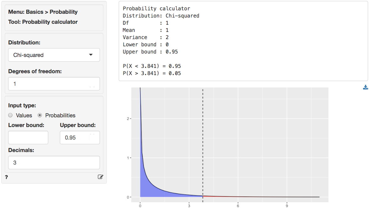
We can use the provided p.value associated with the Chi-squared value of 0.028 to evaluate the null hypothesis. However, we can also calculate the critical Chi-squared value using the probability calculator. As we can see from the output below the critical value is 3.841 if we choose a 95% confidence level. Because the calculated Chi-square value is smaller than the critical value (0.028 < 3.841) we cannot reject null hypothesis stated above.

<p align="center"><img src="https://radiant-rstats.github.io/docs/basics/figures_basics//compare_props_prob_calc.png"></p>

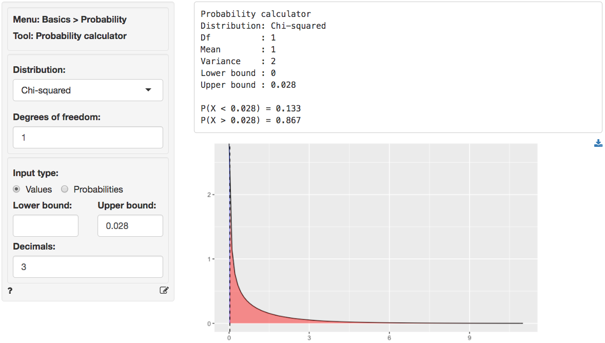
We can also use the probability calculator to determine the p.value associated with the calculated Chi-square value. Consistent with the output from the _Summary_ tab this `p.value` is `< .001`.

<p align="center"><img src="https://radiant-rstats.github.io/docs/basics/figures_basics//goodness_chi_pvalue.png"></p>

In addition to the numerical output provided in the _Summary_ tab we can evaluate the hypothesis visually in the _Plot_.

### Report > Rmd

Add code to <a href="https://radiant-rstats.github.io/docs/data/report_rmd.html" target="_blank">_Report > Rmd_</a> to (re)create the analysis by clicking the <i title="report results" class="fa fa-edit"></i> icon on the bottom left of your screen or by pressing `ALT-enter` on your keyboard. 

If a plot was created it can be customized using `ggplot2` commands (e.g., `plot(result, check = "observed", custom = TRUE) + labs(y = "Percentage")`). See <a href="https://radiant-rstats.github.io/docs/data/visualize.html" target="_blank">_Data > Visualize_</a> for details.

### Technical note

When one or more expected values are small (e.g., 5 or less) the p.value for the Chi-squared test is calculated using simulation methods. If some cells have an expected count below 1 it may be necessary to combine cells/categories.

### R-functions

For an overview of related R-functions used by Radiant to evaluate a discrete probability distribution see <a href = "https://radiant-rstats.github.io/radiant.basics/reference/index.html#section-basics-tables" target="_blank">_Basics > Tables_</a>

The key function from the `stats` package used in the `goodness` tool is `chisq.test`.