> Evaluate model performance for (binary) classification
#### Response variable
Select the outcome, or response, variable of interest. This should be a binary variable, either a factor or an integer with two value (i.e., 0 and 1).
#### Choose level
The level in the response variable that is considered a _success_. For example, a purchase or buyer is equal to "yes".
#### Predictor
Select one or more variables that can be used to _predict_ the chosen level in the response variable. This could be a variable, an RFM index, or predicted values from a model (e.g., from a logistic regression estimated using _Model > Logistic regression (GLM)_ or a Neural Network estimated using _Model > Neural Network_).
#### # quantiles
The number of bins to create.
#### Margin & Cost
To use the `Profit` and `ROME` (Return on Marketing Expenditures) charts, enter the `Margin` for each sale and the estimated `Cost` per contact (e.g., mailing costs or opportunity cost of email or text message). For example, if the margin on a sale is \$10 (excluding the contact cost) and the contact cost is \$1 enter 10 and 1 in the `Margin` and `Cost` input windows.
#### Show results for
If a `filter` is active (e.g., set in the _Data > View_ tab) generate results for `All` data, `Training` data, `Test` data, or `Both` training and test data. If no filter is active calculations are applied to all data.
#### Plots
Generate Lift, Gains, Profit, and/or ROME charts.
### Report > Rmd
Add code to _Report > Rmd_ to (re)create the analysis by clicking the icon on the bottom left of your screen or by pressing `ALT-enter` on your keyboard.
If we create a set of four charts in the _Plots_ tab we can add a title above the group of plots and impose a two-column layout using `patchwork` as follows:
```r
plot(result, plots = c("lift", "gains", "profit", "rome"), custom = TRUE) %>%
wrap_plots(plot_list, ncol = 2) + plot_annotation(title = "Model evaluation")
```
The single plot can be customized using `ggplot2` commands (see example below)). See _Data > Visualize_ for details.
```r
plot(result, plots = "lift", custom = TRUE) +
labs(caption = "Based on data from ...")
```
#### Confusion matrix
Predicted probabilities probabilities selected through `Predictor` are first converted to a class (e.g., a positive or negative outcome) using the values entered in `Margin` and `Cost`. It will be profitable to contact a customer if the predicted probability of response exceeds `Cost / Margin`. For example, if the break-even response rate is 0.1 and the predicted probability of response is 0.25 that customer will be assigned the label _Positive_. If, on the other hand, the predicted probability does not exceed the break-even response rate a customer will be assigned a _Negative_ label.
Once each prediction has been converted to a class label (i.e., Positive or Negative) the result is compared to the values of the response variable. The following key measures are shown in the generated table for each predictor.
Label | Description
------------------------ | ------------------------------------------------------------------
TP (True Positive) | Number of cases where the positive prediction matches the positive outcome in the data
FP (False Positive) | Number of cases with a positive prediction but a negative outcome in the data
TN (True Negative) | Number of cases where the negative prediction matches the negative outcome in the data
FN (False Negative) | Number of cases with a negative prediction but a positive outcome in the data
total | Total number of cases (i.e., TP + FP + TN + FN)
TPR (True Positive Rate) | Proportion of positive outcomes in the data that received a positive prediction (i.e., TP / (TP + FN)). Also known as _sensitivity_ or _recall_
TNR (True Negative Rate) | Proportion of negative outcomes in the data that received a negative prediction (i.e., TN / (TN + FP)). Also known as _specificity_
precision | Proportion of positive predictions with a positive outcome in the data (i.e., TP / (TP + FP))
F-score | The harmonic mean of _precision_ and TPR (_sensitivity_)
accuracy | Proportion of all outcomes that was correctly predicted as either positive or negative (i.e., (TP + TN) / total)
kappa | Corrects the accuracy measure for the probability of generating a correct prediction purely by chance
profit | Total profitability achieved by targeting all customers with a predicted probability above the break-even response rate
index | Index of relative profitability achieved across the selected `Predictor` variables (maximum is 1)
ROME | Return on Marketing Expenditures (ROME) achieved by targeting all customers with a predicted probability above the break-even response rate
contact | Proportion of customers to contact, i.e., (TP + FP) / total
AUC | Area Under the ROC Curve (AUC). ROC stands for Receiver Operating Characteristic.
### Report > Rmd (confusion)
Add code to _Report > Rmd_ to (re)create the analysis by clicking the icon on the bottom left of your screen or by pressing `ALT-enter` on your keyboard.
Only `kappa`, `index`, `ROME`, and `AUC` are plotted by default. It is possible to customize the plotted results through _Report > Rmd_. To change the plot use, for example:
```r
plot(result, vars = c("precision", "profit", "AUC"))
```
The plot can be further customized using `ggplot2` commands (see example below)). See _Data > Visualize_ for details.
```r
plot(result, vars = c("precision", "profit", "AUC")) +
labs(caption = "Based on data from ...")
```
#### Download options
To download a table as a csv-files click the download button on the top-right of your screen. To download plots as png files click the download icon on the middle-right of your screen.
## Example
The Lift and Gains charts below show little evidence of overfitting and suggest that targeting approximately 65% of customers would maximize profits.
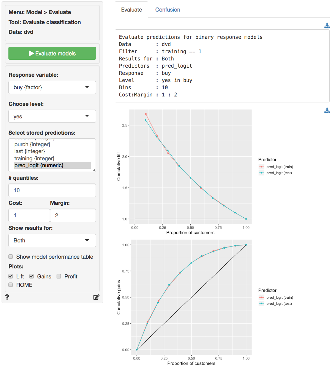
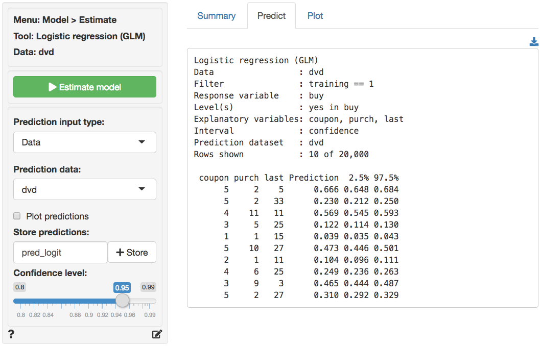
The prediction used in the screen shots above was derived from a logistic regression on the `dvd` data. The data is available through the _Data > Manage_ tab (i.e., choose `Examples` from the `Load data of type` drop-down and press `Load`). The model was estimated using _Model > Logistic regression (GLM)_. The predictions shown below were generated in the _Predict_ tab.
### R-functions
For an overview of related R-functions used by Radiant to evaluate (binary) classification models see _Model > Evaluate classification_