> Compare a single mean to the mean value in the population The single mean (or one-sample) t-test is used to compare the mean of a variable in a sample of data to a (hypothesized) mean in the population from which our sample data are drawn. This is important because we seldom have access to data for an entire population. The hypothesized value in the population is specified in the `Comparison value` box. We can perform either a one-sided test (i.e., `less than` or `greater than`) or a two-sided test (see the `Alternative hypothesis` dropdown). We use one-sided tests to evaluate if the available data provide evidence that the sample mean is larger (or smaller) than the comparison value (i.e., the population value in the null-hypothesis). ## Example We have access to data from a random sample of grocery stores in the UK. Management will consider entering this market if consumer demand for the product category exceeds 100M units, or, approximately, 1750 units per store. The average demand per store in the sample is equal to 1953. While this number is larger than 1750 we need to determine if the difference could be attributed to sampling error. You can find the information on unit sales in each of the sample stores in the **demand\_uk.rda** data set. The data set contains two variables, `store_id` and `demand_uk`. Our null-hypothesis is that the average store demand in the UK is equal to 1750 unit so we enter that number into the `Comparison value` box. We choose the `Greater than` option from the `Alternative hypothesis` drop-down because we want to determine if the available data provides sufficient evidence to reject the null-hypothesis favor of the alternative that average store demand in the UK is **larger than 1750**.

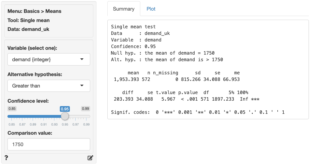
The first two blocks of output show basic information about the test (e.g.,. the null and alternative hypothesis) and summary statistics (e.g., mean, standard deviation, standard error, margin or error, etc.). The final row of output shows the following: * `diff` is the difference between the sample mean (1953.393) and the comparison value (1750) * `se` is the standard error (i.e., the standard deviation of the sampling distribution of `diff`) * `t.value` is the _t_ statistic associated with `diff` that we can compare to a t-distribution (i.e., `diff` / `se`) * `p.value` is the probability of finding a value as extreme or more extreme than `diff` if the null hypothesis is true * `df` is the degrees of freedom associated with the statistical test (i.e., _n_ - 1) * `5% 100%` show the 95% confidence interval around the sample mean (1897 to Inf.). These numbers provide a range within which the true population mean is likely to fall ### Testing There are three approaches we can use to evaluate the null hypothesis. We will choose a significance level of 0.05.¹ Of course, each approach will lead to the same conclusion. #### p.value Because the p.value is **smaller** than the conventional significance level (i.e., 0.05) we reject the null hypothesis and suggest that management should enter the UK market. Note also the '***' that are used as an indicator for significance. #### confidence interval Because the `comparison value` is **not** contained in the confidence interval we reject the null hypothesis and suggest that management should enter the UK market. 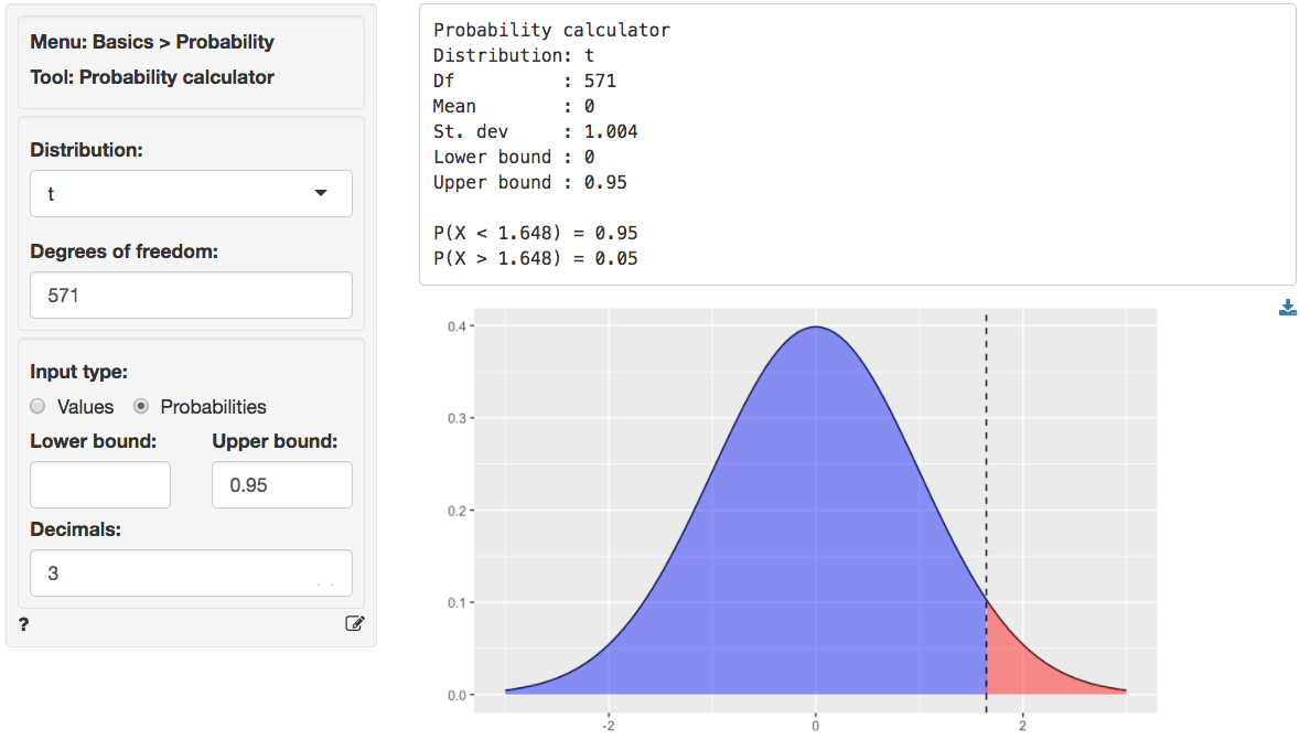#### t.value Because the calculated t.value (5.967) is **larger** than the _critical_ t.value we reject the null hypothesis and suggest that management should enter the UK market. We can obtain the critical t.value by using the probability calculator in the _Basics_ menu. For a t-distribution with 571 degrees of freedom (see `df`) the critical t.value is 1.648. We have to enter 0.95 as the upper probability bound (i.e., 1 - 0.05) because the alternative hypothesis is `Greater than`.²

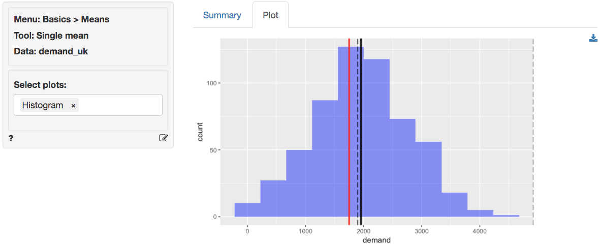
In addition to the numerical output provided in the _Summary_ tab we can visualize the data in the _Plot_ tab. The settings in the side-panel are the same as before. The black lines in the histogram show the sample mean (solid) and the confidence interval around the sample mean (dashed). The red line shows the comparison value (i.e., unit sales under the null-hypothesis). Because the red line does **not** fall within the confidence interval (1897 to Inf.) we reject the null-hypothesis in favor of the alternative.

### _Stats speak_ This is a **single mean** test of the null hypothesis that the true population **mean** is equal to **1750**. Using a significance level of 0.05, we reject the null hypothesis, and conclude that the true population **mean** is **larger** than **1750**. The p.value for this test is **< .001**. This is the probability of observing a sample **mean** that is as or more extreme than the sample **mean** from the data if the null hypothesis is true. In this case, it is the probability of observing a sample **mean** that is larger than (or equal to) **1953.393** if the true population **mean** is **1750**. The 5% confidence bound is **1897.233**. If repeated samples were taken and the 5% confidence bound computed for each one, the true population mean would exceed the lower bound in 95% of the samples ¹ The **significance level**, often denoted by $\alpha$, is the highest probability you are willing to accept of rejecting the null hypothesis when it is actually true. A commonly used significance level is 0.05 (or 5%) ² $1 - \alpha$ is called the **confidence level**. A commonly used confidence level is 0.95 (or 95%) ### Report > Rmd Add code to _Report > Rmd_ to (re)create the analysis by clicking the icon on the bottom left of your screen or by pressing `ALT-enter` on your keyboard. If a plot was created it can be customized using `ggplot2` commands (e.g., `plot(result, plots = "hist", custom = TRUE) + labs(title = "Histogram")`). See _Data > Visualize_ for details. ### R-functions For an overview of related R-functions used by Radiant to evaluate means see _Basics > Means_. The key function from the `stats` package used in the `single_mean` tool is `t.test`. ### Video Tutorials Copy-and-paste the full command below into the RStudio console (i.e., the bottom-left window) and press return to gain access to all materials used in the hypothesis testing module of the Radiant Tutorial Series:

usethis::use_course("https://www.dropbox.com/sh/0xvhyolgcvox685/AADSppNSIocrJS-BqZXhD1Kna?dl=1")

Single Mean Hypothesis Test * This video shows how to test a hypothesis about a single sample mean versus a population mean * Topics List: - Calculate summary statistics for a sample - Setup a hypothesis test for a single mean in Radiant - Use the p.value, confidence interval, or critical value to evaluate the hypothesis test