> Compare proportions for two or more groups in the data The compare proportions test is used to evaluate if the frequency of occurrence of some event, behavior, intention, etc. differs across groups. The null hypothesis for the difference in proportions across groups in the population is set to zero. We test this hypothesis using sample data. We can perform either a one-tailed test (i.e., `less than` or `greater than`) or a two-tailed test (see the `Alternative hypothesis` dropdown). A one-tailed test is useful if we want to evaluate if the available sample data suggest that, for example, the proportion of dropped calls is larger (or smaller) for one wireless provider compared to others. ### Example We will use a sample from a dataset that describes the survival status of individual passengers on the Titanic. The principal source for data about Titanic passengers is the Encyclopedia Titanic. One of the original sources is Eaton & Haas (1994) Titanic: Triumph and Tragedy, Patrick Stephens Ltd, which includes a passenger list created by many researchers and edited by Michael A. Findlay. Lets focus on two variables in the database: - survived = a factor with levels `Yes` and `No` - pclass = Passenger Class (1st, 2nd, 3rd). This is a proxy for socio-economic status (SES) 1st ~ Upper; 2nd ~ Middle; 3rd ~ Lower Suppose we want to test if the proportion of people that survived the sinking of the Titanic differs across passenger classes. To test this hypothesis we select `pclass` as the grouping variable and calculate proportions of `yes` (see `Choose level`) for `survived` (see `Variable (select one)`). In the `Choose combinations` box select all available entries to conduct pair-wise comparisons across the three passenger class levels. Note that removing all entries will automatically select all combinations. Unless we have an explicit hypothesis for the direction of the effect we should use a two-sided test (i.e., `two.sided`). Our first alternative hypothesis would be 'The proportion of survivors among 1st class passengers was different compared to 2nd class passengers'.

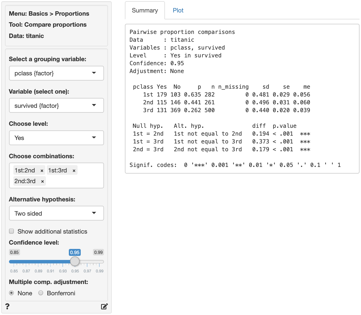
The first two blocks of output show basic information about the test (e.g.,. selected variables and confidence levels) and summary statistics (e.g., proportions, standard error, margin or error, etc. per group). The final block of output shows the following: * `Null hyp.` is the null hypothesis and `Alt. hyp.` the alternative hypothesis * `diff` is the difference between the sample proportion for two groups (e.g., 0.635 - 0.441 = 0.194). If the null hypothesis is true we expect this difference to be small (i.e., close to zero) * `p.value` is the probability of finding a value as extreme or more extreme than `diff` if the null hypothesis is true If we check `Show additional statistics` the following output is added:

Pairwise proportion comparisons
Data      : titanic 
Variables : pclass, survived 
Level     : Yes in survived 
Confidence: 0.95 
Adjustment: None 

 pclass Yes  No     p   n n_missing    sd    se    me
    1st 179 103 0.635 282         0 8.086 0.029 0.056
    2nd 115 146 0.441 261         0 8.021 0.031 0.060
    3rd 131 369 0.262 500         0 9.832 0.020 0.039

 Null hyp.   Alt. hyp.              diff  p.value chisq.value df 2.5%  97.5%    
 1st = 2nd   1st not equal to 2nd   0.194 < .001  20.576      1  0.112 0.277 ***
 1st = 3rd   1st not equal to 3rd   0.373 < .001  104.704     1  0.305 0.441 ***
 2nd = 3rd   2nd not equal to 3rd   0.179 < .001  25.008      1  0.107 0.250 ***

Signif. codes:  0 '***' 0.001 '**' 0.01 '*' 0.05 '.' 0.1 ' ' 1

* `chisq.value` is the chi-squared statistic associated with `diff` that we can compare to a chi-squared distribution. For additional discussion on how this metric is calculated see the help file in _Basics > Tables > Cross-tabs_. For each combination the equivalent of a 2X2 cross-tab is calculated. * `df` is the degrees of freedom associated with each statistical test (1). * `2.5% 97.5%` show the 95% confidence interval around the difference in sample proportions. These numbers provide a range within which the true population difference is likely to fall ### Testing There are three approaches we can use to evaluate the null hypothesis. We will choose a significance level of 0.05.¹ Of course, each approach will lead to the same conclusion. #### p.value Because the p.values are **smaller** than the significance level for each pair-wise comparison we can reject the null hypothesis that the proportions are equal based on the available sample of data. The results suggest that 1st class passengers were more likely to survive the sinking than either 2nd or 3rd class passengers. In turn, the 2nd class passengers were more likely to survive than those in 3rd class. #### Confidence interval Because zero is **not** contained in any of the confidence intervals we reject the null hypothesis for each evaluated combination of passenger class levels. 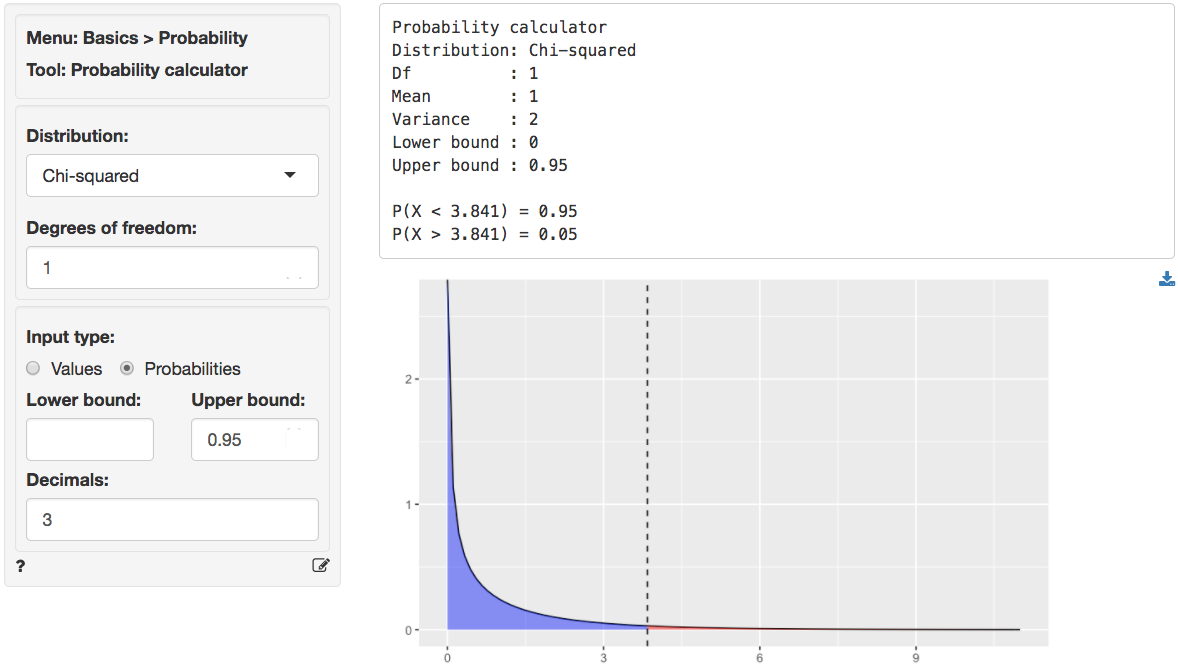#### Chi-squared values Because the calculated chi-squared values (20.576, 104.704, and 25.008) are **larger** than the corresponding _critical_ chi-squared value we reject the null hypothesis for each evaluated combination of passenger class levels. We can obtain the critical chi-squared value by using the probability calculator in the _Basics_ menu. Using the test for 1st versus 2nd class passengers as an example, we find that for a chi-squared distribution with 1 degree of freedom (see `df`) and a confidence level of 0.95 the critical chi-squared value is 3.841.

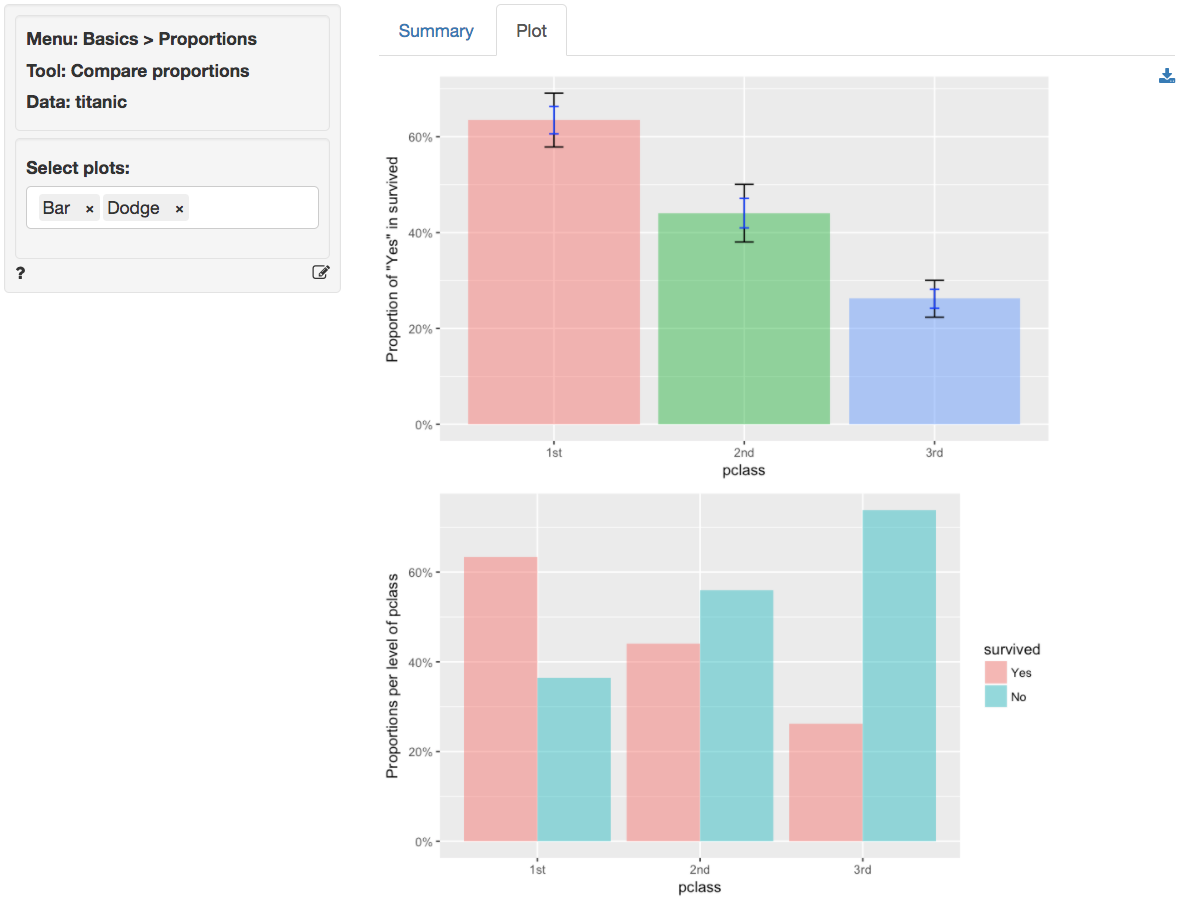
In addition to the numerical output provided in the _Summary_ tab we can also investigate the association between `pclass` and `survived` visually (see the _Plot_ tab). The screen shot below shows two bar charts. The first chart has confidence interval (black) and standard error (blue) bars for the proportion of `yes` entries for `survived` in the sample. Consistent with the results shown in the _Summary_ tab there are clear differences in the survival rate across passenger classes. The `Dodge` chart shows the proportions of `yes` and `no` in `survived` side-by-side for each passenger class. While 1st class passengers had a higher proportion of `yes` than `no` the opposite holds for the 3rd class passengers.

### Technical notes * Radiant uses R's `prop.test` function to compare proportions. When one or more expected values are small (e.g., 5 or less) the p.value for this test is calculated using simulation methods. When this occurs it is recommended to rerun the test using _Basics > Tables > Cross-tabs_ and evaluate if some cells may have an expected value below 1. * For one-sided tests (i.e., `Less than` or `Greater than`) critical values must be obtained by using the normal distribution in the probability calculator and squaring the corresponding Z-statistic. ### Multiple comparison adjustment The more comparisons we evaluate the more likely we are to find a "significant" result just by chance even if the null hypothesis is true. If we conduct 100 tests and set our **significance level** at 0.05 (or 5%) we can expect to find 5 p.values smaller than or equal to 0.05 even if there are no associations in the population. Bonferroni adjustment ensures the p.values are scaled appropriately given the number of tests conducted. This XKCD cartoon expresses the need for this type of adjustments very clearly. ### _Stats speak_ This is a **comparison of proportions** test of the null hypothesis that the true population **difference in proportions** is equal to **0**. Using a significance level of 0.05, we reject the null hypothesis for each pair of passengers classes evaluated, and conclude that the true population **difference in proportions** is **not equal to 0**. The p.value for the test of differences in the survival proportion for 1st versus 2nd class passengers is **< .001**. This is the probability of observing a sample **difference in proportions** that is as or more extreme than the sample **difference in proportions** from the data if the null hypothesis is true. In this case, it is the probability of observing a sample **difference in proportions** that is less than **-0.194** or greater than **0.194** if the true population **difference in proportions** is **0**. The 95% confidence interval is **0.112** to **0.277**. If repeated samples were taken and the 95% confidence interval computed for each one, the true **difference in population proportions** would fall inside the confidence interval in 95% of the samples ¹ The **significance level**, often denoted by $\alpha$, is the highest probability you are willing to accept of rejecting the null hypothesis when it is actually true. A commonly used significance level is 0.05 (or 5%) ### Report > Rmd Add code to _Report > Rmd_ to (re)create the analysis by clicking the icon on the bottom left of your screen or by pressing `ALT-enter` on your keyboard. If a plot was created it can be customized using `ggplot2` commands (e.g., `plot(result, plots = "bar", custom = TRUE) + labs(title = "Compare proportions")`). See _Data > Visualize_ for details. ### R-functions For an overview of related R-functions used by Radiant to evaluate proportions see _Basics > Proportions_. The key function from the `stats` package used in the `compare_props` tool is `prop.test`. ### Video Tutorials Copy-and-paste the full command below into the RStudio console (i.e., the bottom-left window) and press return to gain access to all materials used in the hypothesis testing module of the Radiant Tutorial Series:

usethis::use_course("https://www.dropbox.com/sh/0xvhyolgcvox685/AADSppNSIocrJS-BqZXhD1Kna?dl=1")

Compare Proportions Hypothesis Test * This video shows how to conduct a compare proportions hypothesis test * Topics List: - Setup a hypothesis test for compare means in Radiant - Use the p.value and confidence interval to evaluate the hypothesis test