> Reduce data dimensionality without significant loss of information

As stated in the documentation for pre-factor analysis (see _Multivariate > Factor > Pre-factor_), the goal of factor analysis is to reduce the dimensionality of the data without significant loss of information. The tool tries to achieve this goal by looking for structure in the correlation matrix of the variables included in the analysis. The researcher will often try to link the original variables (or _items_) to an underlying factor and provide a descriptive label for each.

### Example: Toothpaste

First, go to the _Data > Manage_ tab, select **examples** from the `Load data of type` dropdown, and press the `Load` button. Then select the `toothpaste` dataset. The dataset contains information from 60 consumers who were asked to respond to six questions to determine their attitudes towards toothpaste. The scores shown for variables v1-v6 indicate the level of agreement with statements on a 7-point scale where 1 = strongly disagree and 7 = strongly agree.

Once we have determined the number of factors we can extract and rotate them. The factors are rotated to generate a solution where, to the extent possible, a variable has a high loading on only one factor. This is an important benefit because it makes it easier to interpret what the factor represents. While there are numerous algorithms to rotate a factor loadings matrix the most commonly used is Varimax rotation.

To replicate the results shown in the screenshot below make sure you have the `toothpaste` data loaded. Then select variables `v1` through `v6`, set `Nr. of factors` to 2, and press the `Estimate` button or `CTRL-enter` (`CMD-enter` on mac) to generate results.

<p align="center"><img src="https://radiant-rstats.github.io/docs/multivariate/figures_multivariate//full_factor_summary.png"></p>

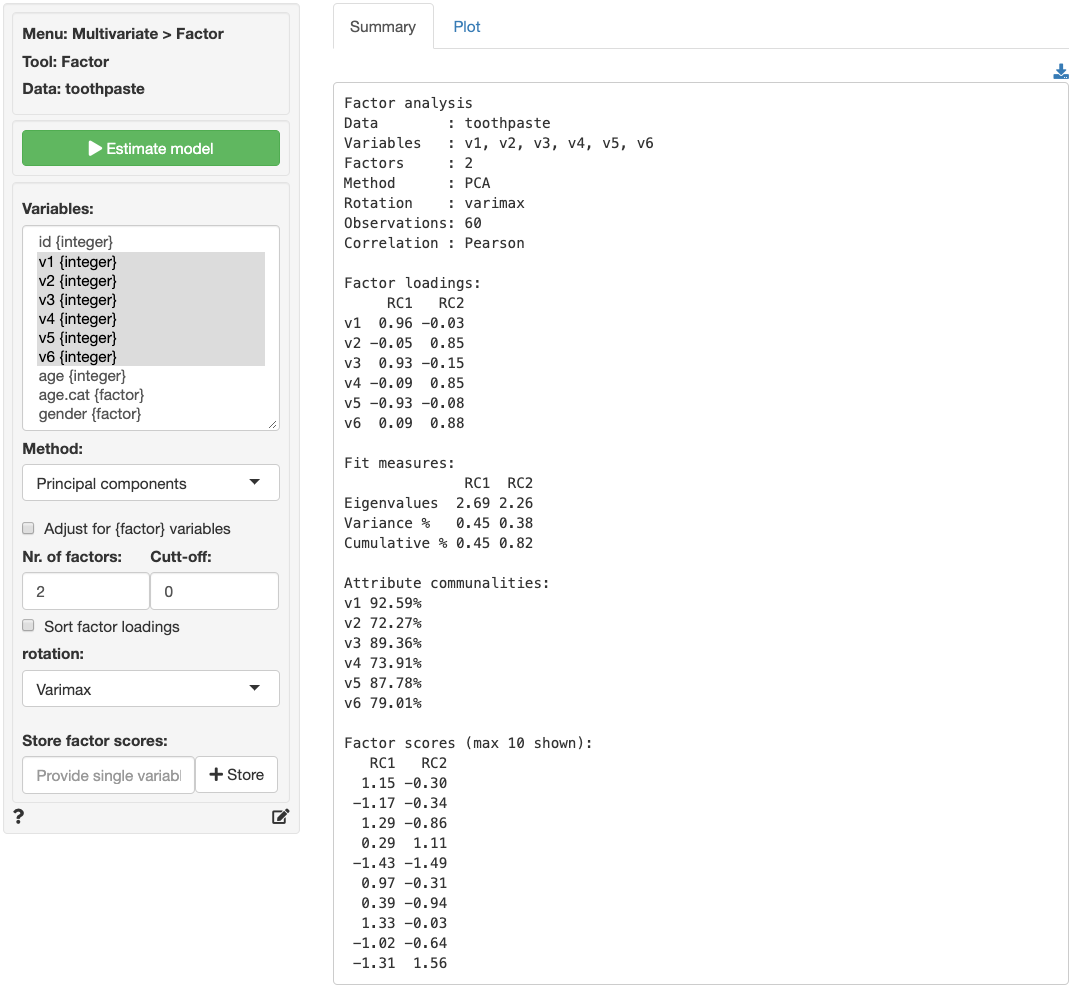
The numbers in the `Factor loadings` table are the correlations of the six variables with the two factors. For example, variable `v1` has a correlation of .96 with factor 1 and a correlation of -.03 with factor 2. As such `v1` will play a big role in naming factor 1 but an insignificant role in naming factor 2.

The rotated factor loadings can be used to determine labels or names for the different factors. We need to identify and highlight the highest factor loading, in absolute value, in each row. This is easily done by setting the `Cut-off` value to .4 and checking the `Sort factor loadings` box. The output is shown below.

```r
Loadings:
     RC1   RC2
v1  0.96
v5 -0.93
v3  0.93
v6        0.88
v4        0.85
v2        0.85
```

Together, the variables shown in each column (i.e., for each factor) help us to understand what the factor represents. Questions 1, 3, and 5 reflect the importance of health issues while questions 2, 4, and 6 reflect aesthetics issues (see the data description in the _Data > Manage_ tab for a description of the variables). Plausible names for the factors might therefore be:

* **Factor 1:** Health benefits
* **Factor 2:** Social benefits

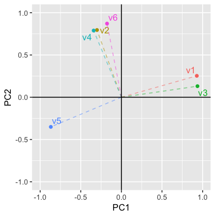
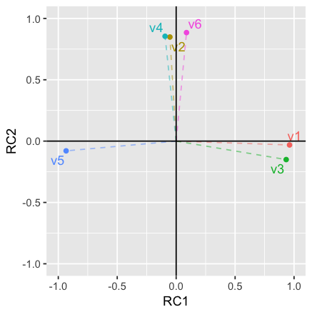
The best way to see what rotation does is to switch between `Varimax` and `None` in the `Rotation` dropdown and inspect what changes in the output after pressing the `Estimate model` button. Select `None` from the `Rotation` dropdown, switch to the _Plot_ tab, and press the `Estimate model` button to see updated results. The image shown below depicts the loadings of the variables on the two factors. Variable `v5` falls somewhat in between the axes for factor 1 and factor 2. When we select `Varimax` rotation, however, the label for `v5` lines up nicely with the horizontal axis (i.e., factor 2). This change in alignment is also reflected in the factor loadings. The unrotated factor loadings for `v5` are -0.87 for factor 1 and -0.35 for factor 2. The rotated factor loadings for `v5` are -0.93 for factor 1 and -0.08 for factor 2.

<p align="center"><img src="https://radiant-rstats.github.io/docs/multivariate/figures_multivariate//full_factor_plot.png"> <img src="https://radiant-rstats.github.io/docs/multivariate/figures_multivariate//full_factor_plot_rotation.png"></p>

The final step is to generate the factor scores. You can think of these scores as a weighted average of the variables that are linked to a factor. They approximate the scores that a respondent would have provided if we could have asked about the factor in a single question, i.e., the respondents inferred ratings on the factors. By clicking on the `Store` button two new variables will be added to the toothpaste data file (i.e., factor1 and factor2). You can see them by going to the _Data > View_ tab. We can use factor scores in other analyses (e.g., cluster analysis or regression). You can rename the new variables, e.g., to `health` and `social` through the _Data > Transform_ tab by selecting `Rename` from the `Transformation type` dropdown.

To download the factor loadings to a csv-file click the download button on the top-right of the screen.

### Summary

1. Determine if the data are appropriate for factor analysis using Bartlett, KMO, and Collinearity (_Multivariate > Factor > Pre-factor_)
2. Determine the number of factors to extract using the scree-plot and eigenvalues > 1 criteria (_Multivariate > Factor > Pre-factor_)
3. Extract the (rotated) factor solution to produce:
	- Factor loadings: Correlations between attributes and factors
	- Factor scores: Inferred ratings on the new factors (i.e., new variables that summarize the original variables)
5. Identify the highest factor loading, in absolute value, in each row (i.e., for each variable)
4. Label the factors using the strongest factor loadings

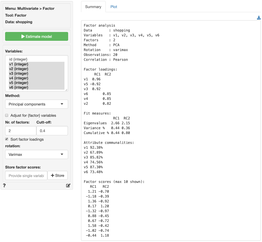
If you want more practice open the `shopping` data set and see if you can reproduce the results shown in the screen capture of the _Summary_ tab below. Use _Multivariate > Factor > Pre-factor_ to determine if the correct number of factors were selected. Do you agree? Why (not)?

<p align="center"><img src="https://radiant-rstats.github.io/docs/multivariate/figures_multivariate//full_factor_summary_shopping.png"></p>

## Including categorical variables

Output shown in _Multivariate > Factor_ is estimated using either Principal Components Analysis (PCA) or Maximum Likelihood (ML). The correlation matrix used as input for estimation can be calculated for variables of type `numeric`, `integer`, `date`, and `factor`. When variables of type factor are included the `Adjust for {factor} variables` box should be checked. When correlations are estimated with adjustment, variables that are of type `factor` will be treated as (ordinal) categorical variables and all other variables will be treated as continuous.

It is important to note that estimated factor scores will be biased if a mixed of {factor} and numeric variables are used. If you want to use factor scores as input for further analysis, e.g., clustering, you should use either (1) all {factor} variables or (2) all numeric variables to avoid this bias.

### Report > Rmd

Add code to <a href="https://radiant-rstats.github.io/docs/data/report_rmd.html" target="_blank">_Report > Rmd_</a> to (re)create the analysis by clicking the <i title="report results" class="fa fa-edit"></i> icon on the bottom left of your screen or by pressing `ALT-enter` on your keyboard. 

If a plot was created it can be customized using `ggplot2` commands or with `patchwork`. See example below and <a href="https://radiant-rstats.github.io/docs/data/visualize.html" target="_blank">_Data > Visualize_</a> for details.

```r
plot(result, custom = TRUE) %>%
  wrap_plots(plot_list, ncol = 2) + plot_annotation(title = "Factor Analysis")
```

### R-functions

For an overview of related R-functions used by Radiant to conduct factor analysis see <a href = "https://radiant-rstats.github.io/radiant.multivariate/reference/index.html#section-multivariate-factor" target="_blank">_Multivariate > Factor_</a>.

The key functions from the `psych` packages used in the `full_factor` tool are `principal` and `fa` .